2# Decision Formulation
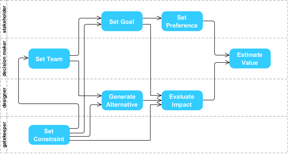
Figure 1.1: Decision Formulation Workflow
Decision formulation is a process of gathering and structuring information to support and make a decision. This includes clarifying roles of decision participants, defining objectives, generating design alternatives, evaluating performance, sorting results and assessing value. This section first provides definitions of the important concepts and processes involved in construction a Design Space based on Clevenger & Haymaker (2011), and then provides an example decision formulation using the Sprout Space case study.
The Organization
A decision is a process that requires many types of expertise, and it is important to identify the participants and their roles. Depending on their role, participants may be affected by decisions, define objectives, apply constraints, or make the decisions. The following questions start to identify all these roles.
Stakeholders
Who are the people, and types of people, who will be affected by the decision? These people will define the Objectives and Preferences of a decision.
Gatekeepers
Who has the ability to restrict the participants, alternatives or goals considered in decisions? These people will be able to place a Constraint on the decision.
Designers
Who are the experts in the domain of the decision? These are people who can help generate Alternatives and measure Impacts of Alternatives on Objectives.
Decision Makers
Who has the power to create the organization and make the decision? These people appoint stakeholders and designers and weigh Value to make decisions.
The Objectives
Objectives are qualitative intents translated into quantitative terms. They can be target-oriented (TO) or failure-preventive (FP) and have specific targets to achieve or failures to avoid. They can be a desirable goal or a mandatory constraint.
Goals
Goals can define specific Experiential, Ecological, or Economic targets. However, in most cases it is impossible to maximize all goals simultaneously and the optimization of a single goal must be compromised in order to maximize overall value. For example, maximizing View Quality (TO), but minimizing Energy Consumption (FP) for heating in the winter or cooling in the summer are both affected by the window/wall ratio of the building envelope. Examples of goals:
- Minimize Energy Consumption
- Maximize Daylight
- Maximize View Quality
Constraints
Constraints are requirements . Alternatives that violate a constraint are not viable. For example, in the Sprout Space case study perhaps the floor area should be a constraint to ensure enough room is provided for the desired program, but not so large that it takes up too much of the site. Use specific units whenever possible. Example of a Constraint:
- At least 75% of all occupied floor area must have a direct line of sight to the outside, according to LEED 4.0.
Providing a larger % of view area might then be formulated as a goal that can be traded off against other Goals.
Metrics
In order to combine multiple Goals and Constraints into a single value function they must be quantifiable. The Metric is the unit in which a Goal or Constraint is quantified. While objectives are declared in qualitative terms, their related indicators are in quantitative ones. The Following metrics are examples that begin to allow the verification of fulfillment of the constraints, and the assessment of the degree of satisfactions of the goals (Table 1.1).
Table 1.1: Quantification of the qualitative objectives
| Objectives | Indicators | Metrics |
|---|---|---|
| Minimize Energy Consumption | Energy Use | W/m2 |
| Maximize Daylight | Daylight Factor | % |
| Maximize Quality View | Quality View (QV) | % |
| Maximize Quality View | Direct Line of Sight (DLS) | % |
Preferences
Goals and Constraints, defined with proper metrics, can begin to be sorted in order of importance, from those that are mandatory to those that are merely desirable. Stakeholders define their unique preferences by prioritizing objectives. Gathering preferences can help drive the formulation, generation and analysis when compromises must occur. Ultimately, a set of design alternatives will be ranked differently depending on the set of Stakeholder Preferences used to evaluate them. Examples of preferences:
- Student: Minimize Energy Consumption 20%, Maximize Daylight 30%, Maximize View Quality 50%
- Teacher: Minimize Energy Consumption 40%, Maximize Daylight 40%, Maximize View Quality 20%
Alternatives
There are many ways to generate a space of Alternatives, including manual, parametric, or generative strategies. This tutorial focuses on parametric modeling.
A parametric model represents a Space of Alternatives by describing a configuration of variables, ranges, and relationships. It assumes that the optimal alternative for a design problem exists within the permutations made possible by the model. It is therefore crucial to define this information collabortively, and iteratively. Finding an optimal solution within these boundaries does not necessarily represent the absolute optimal, since it is only the best design alternative derived from the model. A richer exploration can be achieved by exploring variations of different general configurations and intentionally manipulating the boundaries of the Design Space. Examples of alternatives:
- Alternative 1: Building Orientation = 45, Window Width = 20 ft. (6.09 m.)
- Alternative 2: Building Orientation = 45, Window Width = 15 ft. (4.572 m.)
- Alternative 3: Building Orientation = 30, Window Width = 15 ft. (4.572 m.)
Variables
Variables correspond to the set of inputs that drive the generation of design alternatives. The variables range from those that trigger geometric variation of the parametric model to those that specify attributes required by the analyses such as material properties. Examples of variables:
- Building Orientation (degrees).
- Window Width (ft).
- Wall Construction (Material).
Dependent Variables
In any design space there are relationships between input and derived parameters. Derived parameters depend on input parameters controlling the size of both Wall and Window components. Examples of dependent variables in the Sprout Space model are:
- Floor Area
- Air Volume
Ranges
Ranges define the breadth of acceptable input variable values by defining their lower and upper bounds and increment intervals. Due to the size and complexity of the design spaces, analyzing every possible design alternative can often be an impossible tasks. Specifying the range for each variable makes searching design solutions more efficient. Examples of ranges:
- Building Orientation (degrees) = 45, 30, 15, 0
- Window Width (ft) = 10, 15, 20, 25
Impacts
Once stakeholders have defined objectives and designers have generated alternatives, the next step is to determine the performance impact of each alternative on each Objective (Figure 1.2). The impact is the amount of influence the combined variables in an alternative have on the performance of an objective. Example of impacts of variables over indicators.
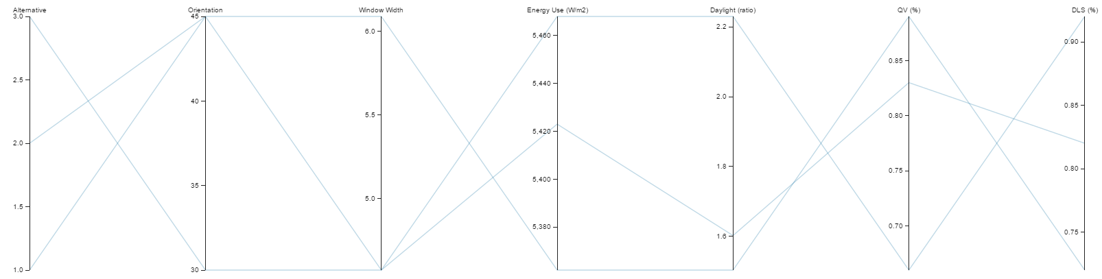
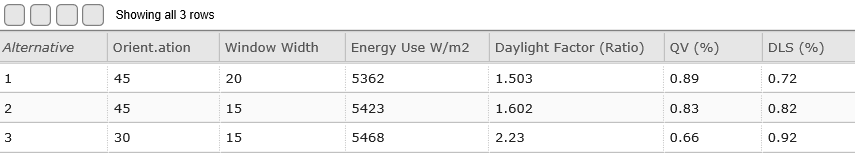
Figure 1.2: Visualization of the impact of the variables on indicators
Value
The next steps require assessment of a Value for every design Alternative so that they can be rationally compared and choices made. Formulation of an effective value function is usually an iterative process of narrowing and expanding the search as decision makers, stakeholders, and designers learn more about the space and their own preferences. Depending of the preferences of the stakeholders and the accuracy of the analysis methods, different alternatives can score the highest value with different levels of certainty of their indicators. The process of sorting and prioritizing the design alternative (Figure 1.3) should include the following steps:
- Ordering of alternatives according to their performance on each objectives
- Ordering of alternatives with respect to goals, priorities, and certainty for each stakeholder
- Ordering of alternatives with respect to goals, priorities, and certainty for all stakeholders
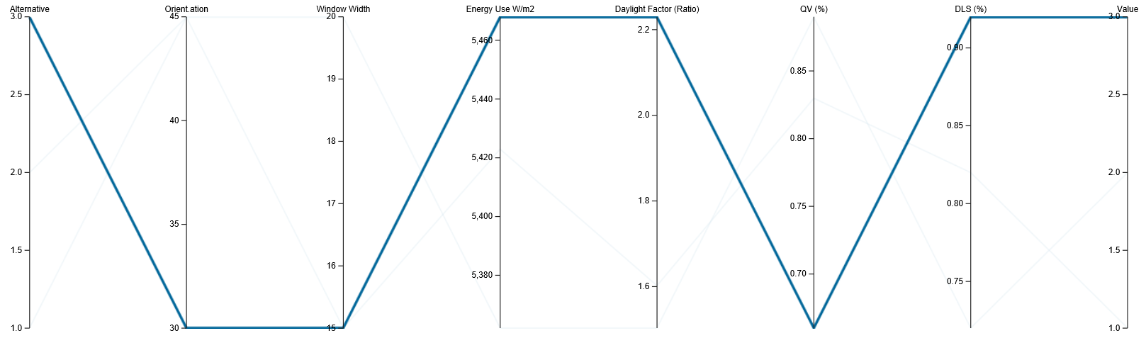
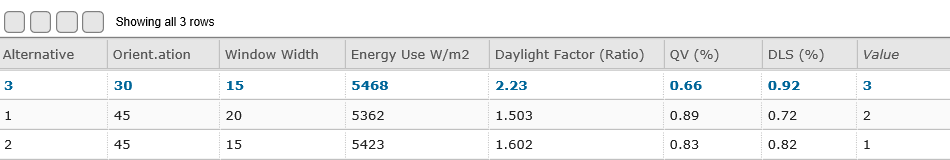
Figure 1.3: Sorted alternatives according to value
Formulation of an effective value function is also a complex topic that can involve optimization, machine learning, uncertainty, and game theory. Therefore this initial e-book stops here, having covered the basic concepts for constructing a design space, and leaving to further chapters to explore extensions of this framework to include more complex aspects of generative design, performance analysis, and decision theory. The next paragraphs apply this formulation of a design space to the design of a relocatable class room.
Case Study: Sprout Space
Sprout Space (Figure 1.4) is a flexible, modular, and mobile class room developed by Perkins + Will. Sprout Space provides the case study to explain a multi-criteria design, optimization and decision making workflow.
- Annual high temperature 71.7 F°
- Annual low temperature 55.9 F°
- Average temperatura 63.8 F°
- Climate zone 3B
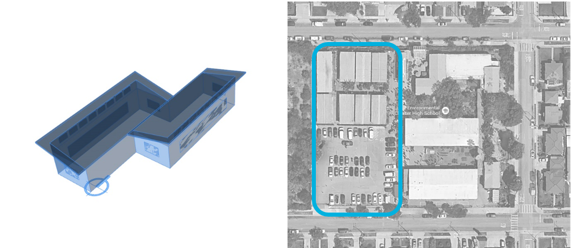
Figure 1.4: Sprout Space, 16315 Grevillea Ave. Los Angeles, CA.
Computational Workflow
The integration of their parametric model with analysis tools allows analyzing, evaluating and visualizing the performances of different alternatives in a design space and compare them based on their performance metrics. The computational workflow (Figure 1.5) has three stages: generation of design alternatives and performance analyses that are based on grasshopper components, and visualization that plots a parallel coordinate chart showing the input variables and the resulting indicator for energy use, daylight factor, direct line of sight and quality view.
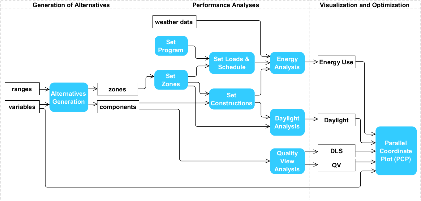
Figure 1.5: The Sprout Space computational workflow.
Geometric Variables
Table 1.2 shows an example of how to define the main driving variables, metrics, their realistic ranges within the theoretical ones, and, in the last column, the number of options of every variable for this case study that combined produce 1296 design alternatives.
Table 1.2: Geometric variables
| Variable | Metrics | Range | Realistic Range | Options |
|---|---|---|---|---|
| Classroom Width | feet | 10 -24 | 12 | 1 |
| Classroom Length | feet | 32 - 42 | 42 | 1 |
| Classroom Height | feet | 10 - 15 | 10 | 1 |
| Classroom Offset | feet | 0 - 60 | 4, 8, 12 | 3 |
| Classroom Orientation | degree | 0-360° | 0, 30, 60, 90, 120, 185 | 6 |
| Front Window Width | feet | 1 - 9 | 1, 2, 3 | 3 |
| Front Window Height | feet | 0.1 - 1.0 | 0.4, 0.7, 1.0 | 3 |
| * Window Wall Ratio Left | % | 0 - 1 | 0.58 | 1 |
| * Window Wall Ratio Right | % | 0 - 1 | 0.411 | 1 |
| Exterior Wall Thickness | feet | 0.5 - 2.0 | 1 | 1 |
| Roof Angle | degree | 0 - 10 | 0.5, 5 | 2 |
| Overhang Depth | feet | 0 - 3 | 0, 1, 2, 3 | 4 |
| Cleresteroy Width | % | 0 - 1.828 | 1.2 | 1 |
| Cleresteroy Height | % | 10 - 75 | 60 | 1 |
| Cleresteroy Spacing | feet | 0 - 1 | 0.142 | 1 |
| Number of Panes | unit | 0 - 12 | 7 | 1 |
Material Properties for LA, CZ3
Table 1.3. Shows the specification of material properties of the componentes of the Sprout Space located in Los Angeles Climate Zone 3 according to the recommendation of ASHRAE 90.1.
Table 1.3: Material properties
| Properties | Imperial Units | option | SI Units | option | Used by |
|---|---|---|---|---|---|
| Front Wall Construction - Walls steel framed (Cavity+continuous insulation) | U-Value (BTU/hr_ft2_F) | 0.07 | U-value (W/m2K) | 0.40 | Energy Model |
| Front Window SHGC | Real Number (0-1) | 0.25 | Real Number (0-1) | 0.25 | Energy Model |
| *Front Window Visual Light Transmittance | Percent 0-100% | 45 | Percent 0-100% | 45.00 | Energy Model |
| Front Window Construction | U-Value (BTU/hr_ft2_F) | 0.5 | U-value (W/m2K) | 2.84 | Energy Model |
| Back Wall Construction - Walls steel framed (Cavity+continuous insulation) | U-Value (BTU/hr_ft2_F) | 0.07 | U-value (W/m2K) | 0.40 | Energy Model |
| Side Wall Construction - Walls steel framed (Cavity+continuous insulation) | U-Value (BTU/hr_ft2_F) | 0.07 | U-value (W/m2K) | 0.40 | Energy Model |
| Side Window SHGC | Real Number (0-1) | 0.25 | Real Number (0-1) | 0.25 | Energy Model |
| *Side Window Visual Light Transmittance | Percent 0-100% | 45 | Percent 0-100% | 45.00 | Energy Model |
| Side Window Construction | U-Value (BTU/hr_ft2_F) | 0.5 | U-value (W/m2K) | 2.84 | Energy Model |
| Roof Construction - Metal (Continuous+cavity insulation) | U-Value (BTU/hr_ft2_F) | 0.04 | U-value (W/m2K) | 1.42 | Energy Model |
| Roof Surface Solar Reflectance | range (0-1) | 0.30 | range (0-1) | 0.30 | Energy Model |
| Roof Surface Thermal Emittance | range (0-1) | 0.90 | range (0-1) | 0.90 | Energy Model |
| Floor Construction - Mass with continuous insulation | U-Value (BTU/hr_ft2_F) | 0.074 | U-value (W/m2K) | 0.42 | Energy Model |
*Min 28%, Preferred 40-60%
Assumptions
Some input variables of the generative and evaluation processes become constants based on assumptions (Table 1.4) usually derived from the regulations and best practices.
Table 1.4: General assumptions
| Variable | Imperial Units | Option | SI Units | option | Used by |
|---|---|---|---|---|---|
| Air Changers Per Hour (Infiltration) | ac/hr | 0.6 | ac/hr | 0.60 | Energy Model |
| Ventilation Rate per Area | cfm/ft2 | 0.117884972 | m3/m2S | 0.0006 | Energy Model |
| Ventilation Rate per Person | cfm/ft2 | 0.982374768 | m3/m2S | 0.005 | Energy Model |
| Lighting Power Density | w/sf | 0.87 | W/m2 | 9.36 | Energy Model |
| Occupancy Schedule | Seasonal, Annual, School Year, Daily, Weekend | Seasonal, Annual, School Year, Daily, Weekend | Energy Model | ||
| Electric Plug Loads | w/sf | 0.929 | W/m2 | 10.00 | Energy Model |
| HVAC heating set point | °F | 64 | °C | 18.00 | Energy Model |
| HVAC cooling set point | °F | 79 | °C | 26.00 | Energy Model |
| HVAC heating setback set point | °F | 73 | °C | 12.00 | Energy Model |
| HVAC cooling setback set point | °F | 90 | °C | 32.00 | Energy Model |
| *Baseline HVAC System | hybrid system | hybrid system | Energy Model | ||
| **Wall Reflectance | 0-100% | 70% | 0-100% | 0.70 | Daylight & Energy |
| **Ceiling Reflectance | 0-100% | 70-90% | 0-100% | 70-90% | Daylight & Energy |
| **Floor Reflectance | 0-100% | 20% | 0-100% | 0.20 | Daylight & Energy |
*For the purpose of this study a simplified HVAC was specified which no heating limit capacity and no cooling limit - This unit can be thought of an ideal unit that mixes zone air with the specified amount of outdoor air and then adds or removes heat and moisture at 100% efficiency in order to meet the specified controls. Therefore, the option is Hybrid Natural Ventilation with Default HVAC Cooling System.